Generative pre-trained transformer (GPT)
![]()
The Genesis of GPT
The GPT series is based on the Transformer architecture, introduced by Vaswani et al. in 2017. Transformers rely on self-attention mechanisms to process sequences of words, enabling them to handle dependencies between distant words in a text effectively. This approach marked a significant departure from previous RNN/CNN architectures, which struggled with long-range dependencies due to their sequential processing nature.
GPT-1: The Foundation
GPT-1, the first in the series, demonstrated the viability of using unsupervised pre-training followed by supervised fine-tuning for NLP tasks. With 117 million parameters, GPT-1 was trained on the BooksCorpus dataset, which contains over 7,000 unpublished books. This model laid the groundwork for its successors by showcasing the potential of transformer-based architectures in generating coherent text.
GPT-2: A Leap Forward
Architecture

GPT-2, a direct scale-up of GPT-1, boasts a significantly larger architecture with 1.5 billion parameters, making it one of the largest models of its time. It utilizes 48 layers of transformers with a hidden size of 1600, organized into 12 attention heads. This deep neural network structure allows GPT-2 to capture complex language patterns and generate high-quality text .
Training
The training of GPT-2 involved a massive corpus known as WebText. This dataset was curated by scraping web pages linked from Reddit posts with at least three upvotes. The final dataset consisted of about 40 GB of text after cleaning and deduplication. The transformer architecture’s ability to handle massive parallelization enabled efficient training on this large dataset .
Capabilities
GPT-2’s capabilities are diverse and impressive. It can generate coherent and contextually relevant text, perform language translation, summarize articles, and answer questions based on provided text. Its text generation is often indistinguishable from human-written content, although it can become repetitive or nonsensical over extended outputs .
The GPT-2 Tokenizer
The GPT-2 tokenizer uses Byte Pair Encoding (BPE), a subword tokenization method. BPE starts with individual characters as the base vocabulary and iteratively merges the most frequent pairs of tokens to form subwords. This approach helps in handling rare and out-of-vocabulary words by breaking them into smaller, more frequent subwords.
GPT-2 Model Sizes

The GPT-2 model comes in four distinct sizes, each defined by the number of parameters they contain:
- GPT-2 Small (124M): This is the smallest variant with 124 million parameters. It serves as a baseline for the GPT-2 family and is suitable for tasks that do not require extensive computational resources.
- GPT-2 Medium (355M): With 355 million parameters, this version strikes a balance between performance and resource requirements, providing improved capabilities over the small version .
- GPT-2 Large (774M): This model, containing 774 million parameters, offers significantly enhanced text generation capabilities compared to the smaller versions. It is often used for more demanding applications where better quality text generation is crucial.
- GPT-2 XL (1.5B): The largest publicly released version of GPT-2, with 1.5 billion parameters, provides the best performance among the GPT-2 models. It can generate high-quality, coherent, and contextually relevant text, making it suitable for advanced research and application in various fields.
Key Modifications in GPT 2 :
In this implementation of GPT-2 , several modifications were made to enhance performance and training efficiency.
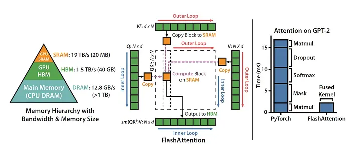
Notably, Flash Attention was incorporated, a technique that optimizes attention computation by using a block-wise approach and leveraging GPU memory hierarchy, significantly reducing memory usage and computational complexity for longer sequences.
Gradient clipping was implemented to prevent exploding gradients, ensuring more stable training.

The model’s weight initialization followed best practices derived from the GPT-3 paper, potentially improving convergence and overall performance. Additionally, a learning rate scheduler combining warmup and cosine decay was employed. This scheduler gradually increases the learning rate during the initial training phase (warmup) to prevent early overfitting, followed by a cosine decay that smoothly reduces the learning rate over time, often leading to better convergence and generalization.

Automatic Mixed Precision (AMP) in PyTorch is a technique to improve the performance of deep learning models by utilizing both 16-bit (half-precision) and 32-bit (single-precision) floating point computations. This approach helps in speeding up training and inference while reducing the memory footprint without compromising model accuracy significantly.

Code Time
Load The Dataset
import pandas as pd

splits = {'v1': 'data/v1-00000-of-00001.parquet'}
df = pd.read_parquet("hf://datasets/ayoubkirouane/Algerian-Darija/" + splits["v1"])
text = df['Text'].to_list()

with open('data.txt', 'w') as f:
  f.write('\n'.join(text))
The code loads our dataset from Hugging Face using pandas. It reads a Parquet file, extracts the Text column, and saves all the text entries to a file called data.txt. Each piece of text is put on its own line. This sets up the raw text data so it’s ready for the next steps in training our Darija-GPT model.
Create our Tokenizer
# Define a generator function to read text data in batches from a file
def text_iterator(file_path, batch_size=1000):
    # Open the file in read mode with UTF-8 encoding
    with open(file_path, 'r', encoding='utf-8') as file:
        batch = []  # Initialize an empty list to store the batch of lines
        # Iterate over each line in the file
        for line in file:
            batch.append(line.strip())  # Strip any leading/trailing whitespace and add the line to the batch
            # If the batch size is reached, yield the batch and reset the batch list
            if len(batch) == batch_size:
                yield batch
                batch = []
        # Yield any remaining lines in the batch that didn't reach the batch size
        if batch:
            yield batch

# Import the AutoTokenizer class from the transformers library
from transformers import AutoTokenizer

# Load the pre-trained GPT-2 tokenizer
tokenizer = AutoTokenizer.from_pretrained("gpt2")

# Train a new tokenizer on the Algerian Darija text data using the text_iterator function
darija_tokenizer = tokenizer.train_new_from_iterator(text_iterator(file_path="data.txt"),
                                                     vocab_size=25000)

# Save the newly trained Darija tokenizer to a directory
darija_tokenizer.save_pretrained("darija_tokenizer")
This code creates a custom tokenizer. It defines a function to read text in batches, then uses the GPT-2 tokenizer as a starting point to train a new tokenizer on our dataset. The new tokenizer, with a vocabulary size of 25,000, is then saved for later use in the model.
GPT Configuration
# Importing necessary libraries
import time
import torch
import torch.nn as nn
from torch.nn import functional as F
from dataclasses import dataclass

# This dictionary contains the configuration parameters for different versions of the GPT-2 model
# The parameters include the number of layers, the number of attention heads, and the embedding dimension
# The numbers provided are for the 'gpt2-large' model
"""
{
    'gpt2':         dict(n_layer=12, n_head=12, n_embd=768),  # 124M params
    'gpt2-medium':  dict(n_layer=24, n_head=16, n_embd=1024), # 350M params
    'gpt2-large':   dict(n_layer=36, n_head=20, n_embd=1280), # 774M params
    'gpt2-xl':      dict(n_layer=48, n_head=25, n_embd=1600), # 1558M params
}
"""

# The GPTConfig class is a data class that holds the configuration parameters for the GPT-2 model
# The parameters are initialized with the values for the 'gpt2-large' model
@dataclass
class GPTConfig:
    block_size: int = 1024  # The maximum context length for the model
    vocab_size: int = 50257  # The size of the vocabulary
    n_layer: int = 36  # The number of layers in the model
    n_head: int = 20  # The number of attention heads in each layer
    n_embd: int = 1280  # The embedding dimension
This code defines a configuration class for the GPT-2 model. The GPTConfig class is a data class that holds the configuration parameters for the model. The parameters include the maximum context length (block_size), the size of the vocabulary (vocab_size), the number of layers (n_layer), the number of attention heads (n_head), and the embedding dimension (n_embd). The values provided are for the gpt2-large model.
Multi-Layer Perceptron (MLP) module
# The MLP class defines a multi-layer perceptron (MLP) module for the GPT-2 model
class MLP(nn.Module):
    # The __init__ method initializes the MLP module with the given configuration
    def __init__(self, config):
        super().__init__()
        # The first linear layer (c_fc) takes the input embedding and maps it to a higher-dimensional space
        self.c_fc = nn.Linear(config.n_embd, 4 * config.n_embd)
        # The gelu activation function is applied to the output of the first linear layer
        self.gelu = nn.GELU(approximate='tanh')
        # The second linear layer (c_proj) maps the output of the gelu activation function back to the original embedding dimension
        self.c_proj = nn.Linear(4 * config.n_embd, config.n_embd)
        # The NANOGPT_SCALE_INIT attribute is set to 1 to scale the output of the second linear layer
        self.c_proj.NANOGPT_SCALE_INIT = 1

    # The forward method defines the forward pass of the MLP module
    def forward(self, x):
        # The input is passed through the first linear layer
        x = self.c_fc(x)
        # The output of the first linear layer is passed through the gelu activation function
        x = self.gelu(x)
        # The output of the gelu activation function is passed through the second linear layer
        x = self.c_proj(x)
        # The output of the second linear layer is returned as the output of the MLP module
        return x
The MLP multi-layer perceptron (MLP) class is a subclass of nn.Module and defines the structure and forward pass of the MLP module. The module consists of a first linear layer (c_fc), a gelu activation function (gelu), and a second linear layer (c_proj).
The forward method defines the forward pass of the MLP module, which takes an input embedding x, passes it through the first linear layer, applies the gelu activation function, passes the output through the second linear layer, and returns the output as the output of the MLP module.
Causal Self Attention
# The CausalSelfAttention class defines a causal self-attention module for the GPT-2 model
class CausalSelfAttention(nn.Module):
    # The __init__ method initializes the causal self-attention module with the given configuration
    def __init__(self, config):
        super().__init__()
        # Assert that the embedding dimension is divisible by the number of attention heads
        assert config.n_embd % config.n_head == 0
        # The c_attn linear layer computes the query, key, and value vectors for all attention heads in batch
        self.c_attn = nn.Linear(config.n_embd, 3 * config.n_embd)
        # The c_proj linear layer computes the output projection of the attention module
        self.c_proj = nn.Linear(config.n_embd, config.n_embd)
        # The NANOGPT_SCALE_INIT attribute is set to 1 to scale the output of the c_proj linear layer
        self.c_proj.NANOGPT_SCALE_INIT = 1
        # The number of attention heads and the embedding dimension are stored as attributes of the module
        self.n_head = config.n_head
        self.n_embd = config.n_embd

    # The forward method defines the forward pass of the causal self-attention module
    def forward(self, x):
        # The input is expected to have shape (B, T, C), where B is the batch size, T is the sequence length, and C is the embedding dimensionality
        B, T, C = x.size()
        # The c_attn linear layer is applied to the input to compute the query, key, and value vectors for all attention heads in batch
        qkv = self.c_attn(x)
        # The query, key, and value vectors are split along the channel dimension
        q, k, v = qkv.split(self.n_embd, dim=2)
        # The key and query vectors are reshaped to have shape (B, nh, T, hs), where nh is the number of attention heads and hs is the head size
        k = k.view(B, T, self.n_head, C // self.n_head).transpose(1, 2)
        q = q.view(B, T, self.n_head, C // self.n_head).transpose(1, 2)
        # The value vectors are reshaped to have shape (B, nh, T, hs)
        v = v.view(B, T, self.n_head, C // self.n_head).transpose(1, 2)
        # The scaled dot-product attention is computed using the query, key, and value vectors
        y = F.scaled_dot_product_attention(q, k, v, is_causal=True) # Flash attention
        # The output of the attention module is reshaped to have shape (B, T, C)
        y = y.transpose(1, 2).contiguous().view(B, T, C)
        # The output projection is computed using the c_proj linear layer
        y = self.c_proj(y)
        # The output of the causal self-attention module is returned
        return y
The CausalSelfAttention class is a subclass of nn.Module and defines the structure and forward pass of the causal self-attention module. The module consists of a linear layer (c_attn) that computes the query, key, and value vectors for all attention heads in batch, and a linear layer (c_proj) that computes the output projection of the attention module.
The forward method defines the forward pass of the causal self-attention module, which takes an input embedding x, computes the query, key, and value vectors for all attention heads in batch using the c_attn linear layer, computes the scaled dot-product attention using the query, key, and value vectors, computes the output projection using the c_proj linear layer, and returns the output of the causal self-attention module.
Decoder Block
The DecoderBlock class is a subclass of nn.Module and defines the structure and forward pass of the decoder block. The block consists of a causal self-attention module (attn) and a multi-layer perceptron module (mlp), both of which are preceded by layer normalization layers (ln_1 and ln_2).
# The DecoderBlock class defines a decoder block for the GPT-2 model
class DecoderBlock(nn.Module):
    # The __init__ method initializes the decoder block with the given configuration
    def __init__(self, config):
        super().__init__()
        # The first layer normalization layer (ln_1) is applied to the input before the causal self-attention module
        self.ln_1 = nn.LayerNorm(config.n_embd)
        # The causal self-attention module (attn) computes the attention weights for the input sequence
        self.attn = CausalSelfAttention(config)
        # The second layer normalization layer (ln_2) is applied to the input before the multi-layer perceptron module
        self.ln_2 = nn.LayerNorm(config.n_embd)
        # The multi-layer perceptron module (mlp) computes the output of the decoder block
        self.mlp = MLP(config)

    # The forward method defines the forward pass of the decoder block
    def forward(self, x):
        # The input is passed through the causal self-attention module, with layer normalization applied to the input before the module
        x = x + self.attn(self.ln_1(x))
        # The output of the causal self-attention module is passed through the multi-layer perceptron module, with layer normalization applied to the input before the module
        x = x + self.mlp(self.ln_2(x))
        # The output of the decoder block is returned
        return x

The forward method defines the forward pass of the decoder block, which takes an input embedding x, passes it through the causal self-attention module with layer normalization applied to the input before the module, passes the output through the multi-layer perceptron module with layer normalization applied to the input before the module, and returns the output of the decoder block.
Data Loader
# The DataLoader class defines a data loader for the GPT-2 model
class DataLoader:
    # The __init__ method initializes the data loader with the batch size (B) and the sequence length (T)
    def __init__(self, B, T):
        self.B = B
        self.T = T

        # Open the data file and read the text
        with open('data.txt', 'r') as f:
            text = f.read()

        # Tokenize the text using the darija_tokenizer
        tokens = darija_tokenizer.encode(text)

        # Convert the tokens to a PyTorch tensor
        self.tokens = torch.tensor(tokens)

        # Initialize the current position to 0
        self.current_position = 0

    # The next_batch method returns the next batch of data
    def next_batch(self):
        # Get the batch size (B) and the sequence length (T)
        B, T = self.B, self.T

        # Get the next batch of tokens from the current position
        buf = self.tokens[self.current_position: self.current_position + B * T + 1]

        # Split the batch of tokens into input (x) and target (y) sequences
        x = (buf[:-1]).view(B, T)
        y = (buf[1:]).view(B, T)

        # Update the current position
        self.current_position += T * B

        # If the current position is beyond the end of the data, reset it to 0
        if self.current_position + (B * T + 1) > len(self.tokens):
            self.current_position = 0

        # Return the input and target sequences
        return x, y
The DataLoader class is initialized with the batch size (B) and the sequence length (T). The next_batch method returns the next batch of data, which consists of input and target sequences.
The input sequence is obtained by taking a slice of the tokens tensor starting from the current position and reshaping it to have shape (B, T). The target sequence is obtained by taking a slice of the tokens tensor starting from the current position plus one and reshaping it to have shape (B, T).
The current position is then updated by adding T * B to it. If the current position is beyond the end of the data, it is reset to 0.
GPT-2 model
class GPT(nn.Module):
    def __init__(self, config):
        super().__init__()
        self.config = config
        # The transformer module consists of the token embedding layer (wte), the positional embedding layer (wpe), the decoder blocks (h), and the final layer normalization layer (ln_f)
        self.transformer = nn.ModuleDict(dict(
            wte = nn.Embedding(config.vocab_size, config.n_embd),  # Token Embedding
            wpe = nn.Embedding(config.block_size, config.n_embd) , # Positional Encoding
            h = nn.ModuleList([DecoderBlock(config) for _ in range(config.n_layer)]), # The Decoder Block
            ln_f = nn.LayerNorm(config.n_embd ) # Layer Normalization
        ))

        # output projection
        self.lm_head = nn.Linear(config.n_embd, config.vocab_size , bias=False)


        # weight sharing
        self.transformer.wte.weight = self.lm_head.weight

        # Weight sharing between the token embedding layer and the output projection layer (from the paper)
        self.apply(self._init_weights)

    # The _init_weights method initializes the weights of the model
    def _init_weights(self, module):
        if isinstance(module, nn.Linear):
            std = 0.02
            if hasattr(module, 'NANOGPT_SCALE_INIT'):
                std *= (2 * self.config.n_layer) ** -0.5
            torch.nn.init.normal_(module.weight, mean=0.0, std=std)
            if module.bias is not None:
                torch.nn.init.zeros_(module.bias)
        elif isinstance(module, nn.Embedding):
            torch.nn.init.normal_(module.weight, mean=0.0, std=0.02)

    # the Forward
    def forward(self, idx , target=None):
      B, T = idx.size()
      assert T <= self.config.block_size, f"Cannot forward sequence of size {T}, block size is only {self.config.block_size}"
      pos = torch.arange(0, T, dtype=torch.long, device=device)
      pos_embed = self.transformer.wpe(pos) # positional embedding
      tok_embed = self.transformer.wte(idx) # token embedding
      x = tok_embed + pos_embed

      # forward the blocks ofthe transformer

      for block in self.transformer.h:
        x = block(x)

      # forward the final LayerNorm and the classifier

      x = self.transformer.ln_f(x)
      loss = None
      logits = self.lm_head(x)
      # Calculate the loss
      if target is not None:
        loss = F.cross_entropy(logits.view(-1, logits.size(-1)), target.view(-1))
      return logits , loss
The GPT model consists of a transformer module (transformer) and an output projection layer (lm_head).
The transformer module consists of the token embedding layer (wte), the positional embedding layer (wpe), the decoder blocks (h), and the final layer normalization layer (ln_f).
The output projection layer maps the output of the transformer to the vocabulary space.
The forward method defines the forward pass of the model, which takes an input sequence idx and an optional target sequence target, generates the positional embedding and the token embedding for the input sequence, passes the input through the decoder blocks of the transformer, passes the output of the transformer through the final layer normalization layer, passes the output of the final layer normalization layer through the output projection layer to obtain the logits, calculates the loss using cross-entropy loss if the target sequence is provided, and returns the logits and the loss.
Create The model and compile it
# Set the device to use for training the model
device = torch.device('cuda' if torch.cuda.is_available() else 'cpu')

# Create an instance of the GPT-2 model with the default configuration
model = GPT(GPTConfig())

# Set the model to evaluation mode
model.eval()

# Move the model to the device
model.to(device)

# Compile the model using PyTorch's just-in-time compiler
model = torch.compile(model)
This code sets the device to use for training the model, creates an instance of the GPT-2 model with the default configuration, sets the model to evaluation mode, moves the model to the device, and compiles the model using PyTorch’s just-in-time compiler.
torch.compile makes PyTorch code run faster by JIT-compiling PyTorch code into optimized kernels, all while requiring minimal code changes.
torch.set_float32_matmul_precision('high')
Running float32 matrix multiplications in lower precision may significantly increase performance, and in some programs the loss of precision has a negligible impact.
highfloat32 matrix multiplications either use the TensorFloat32 datatype (10 mantissa bits explicitly stored) or treat each float32 number as the sum of two bfloat16 numbers (approximately 16 mantissa bits with 14 bits explicitly stored), if the appropriate fast matrix multiplication algorithms are available. Otherwise float32 matrix multiplications are computed as if the precision is “highest”.
optimizer = torch.optim.AdamW(model.parameters(),
                              lr=3e-4 ,
                              betas=(0.9, 0.95) ,
                              eps=1e-8)
Creates an instance of the AdamW optimizer that can be used to train the model with weight decay and a learning rate of lr=3e-4 , betas=(0.9, 0.95) , eps=1e-8.
The learning rate determines how quickly the model learns, while the beta coefficients and epsilon value control the behavior of the optimizer. It’s important to choose appropriate values for these hyperparameters based on the specific problem and model architecture.
Learning rate scheduler
import math

max_lr = 6e-4
min_lr = max_lr * 0.1 # 10 %
warmup_steps = 10
max_steps = 1000

def get_lr(step):
    if step < warmup_steps:
        return max_lr * (step + 1) / warmup_steps
    if step  > max_steps:
        return min_lr
    decay_ratio = (step - warmup_steps) / (max_steps - warmup_steps)
    assert 0 <= decay_ratio <= 1

    coeff = 0.5 * (1.0 + math.cos(math.pi * decay_ratio))
    return min_lr + coeff * (max_lr - min_lr)
The learning rate scheduler is used to adjust the learning rate during training to improve convergence and avoid overshooting the optimal solution.
The warmup phase linearly increases the learning rate from 0 to max_lr over the first warmup_steps steps, which can help to improve convergence when training with large batch sizes.
The cosine decay phase then gradually decreases the learning rate from max_lr to min_lr over the remaining training steps, which can help to prevent overshooting the optimal solution.
Start Training
# Create an instance of the DataLoader class with a batch size of 4 and a sequence length of 128
train_loader = DataLoader(B=4, T=128)
save_interval = 500

# Loop over the maximum number of training steps
for step in range(max_steps):
    # Record the start time of the current training step
    t0 = time.time()

    # Get the next batch of data from the DataLoader
    x, y = train_loader.next_batch()

    # Move the input and target sequences to the device (GPU if available, otherwise CPU)
    x = x.to(device)
    y = y.to(device)

    # Zero out the gradients of the optimizer
    optimizer.zero_grad()

    # Uncomment the following lines to enable automatic mixed precision training
    # with torch.autocast(device_type=device, dtype=torch.bfloat16):
    #     logits, loss = model(x, y)

    # Forward propagate the input sequence through the model and calculate the loss
    logits, loss = model(x, y)

    # Backpropagate the loss through the model to calculate the gradients
    loss.backward()

    # Clip the gradients to a maximum norm of 1.0 to prevent exploding gradients
    norm = torch.nn.utils.clip_grad_norm_(model.parameters(), 1.0)

    # Get the learning rate for the current training step using the learning rate scheduler
    lr = get_lr(step)

    # Update the learning rate for each parameter group in the optimizer
    for param_group in optimizer.param_groups:
        param_group['lr'] = lr

    # Update the model's parameters using the optimizer
    optimizer.step()

    # Wait for the GPU to finish any remaining work
    torch.cuda.synchronize()

    # Record the end time of the current training step
    t1 = time.time()

    # Calculate the time difference between the start and end of the current training step
    dt = (t1 - t0) * 1000

    # Calculate the number of tokens processed per second
    tokens_per_sec = (train_loader.B * train_loader.T) / (t1 - t0)

    # Print the current training step, loss, time difference, gradient norm, and tokens processed per second
    print(f"step {step}, loss: {loss.item()}, dt: {dt:.2f}ms, norm : {norm:.4f} ,tok/sec: {tokens_per_sec:.2f}")
    # Save the model periodically
    if (step + 1) % save_interval == 0:
        torch.save(model.state_dict(), f'model_step_{step + 1}.pt')
        print(f"Model saved at step {step + 1}")

    # Save the final model
    torch.save(model.state_dict(), 'model_final.pt')
    print("Final model saved")
It loops over the maximum number of training steps, and in each step, it gets the next batch of data from the DataLoader, moves the input and target sequences to the device, zeroes out the gradients of the optimizer, forwards propagates the input sequence through the model and calculates the loss, backpropagates the loss through the model to calculate the gradients, clips the gradients to prevent exploding gradients, updates the learning rate for each parameter group in the optimizer, updates the model’s parameters using the optimizer, waits for the GPU to finish any remaining work, calculates the time difference between the start and end of the current training step, calculates the number of tokens processed per second, and prints the current training step, loss, time difference, gradient norm, and tokens processed per second.
Inference phase
# Set the maximum length of the generated text to 30
max_length = 30

# Set the number of sequences to generate to 5
num_return_sequences = 5

# Tokenize the input text "وحد نهار" using the new_tokenizer and convert it to a PyTorch tensor
tokens = darija_tokenizer.encode("وحد نهار")
tokens = torch.tensor(tokens, dtype=torch.long)

# Add a batch dimension to the input tensor and repeat it num_return_sequences times to generate multiple sequences
tokens = tokens.unsqueeze(0).repeat(num_return_sequences, 1)

# Move the input tensor to the device (GPU if available, otherwise CPU)
x = tokens.to(device)

while x.size(1) < max_length:
    # forward the model to get the logits
    with torch.no_grad():
        outputs = model(x) # (B, T, vocab_size)
        # take the logits at the last position
        logits = outputs[0] if isinstance(outputs, tuple) else outputs
        logits = logits[:, -1, :] # (B, vocab_size)
        # get the probabilities
        probs = F.softmax(logits, dim=-1)
        # topk_probs here becomes (5, 50), topk_indices is (5, 50)
        topk_probs, topk_indices = torch.topk(probs, 50, dim=-1)
        # select a token from the top-k probabilities
        # note: multinomial does not demand the input to sum to 1
        ix = torch.multinomial(topk_probs, 1) # (B, 1)
        # gather the corresponding indices
        xcol = torch.gather(topk_indices, -1, ix) # (B, 1)
        # append to the sequence
        x = torch.cat((x, xcol), dim=1)

# print the generated text
for i in range(num_return_sequences):
    tokens = x[i, :max_length].tolist()
    decoded = darija_tokenizer.decode(tokens)
    print(">", decoded)
The code generates 5 different sequences starting with the input text وحد نهار, and each sequence is generated by repeatedly sampling from the model’s probability distribution over the vocabulary until the maximum length is reached. The generated sequences can be used for various purposes, such as generating responses to user input, generating text for a language model, or generating data for training other models.