Mixture of Experts
Mixture of experts (moe) is an advanced neural network architecture designed to enhance model performance by leveraging a diverse set of specialized sub-networks known as "experts" , the core idea is to dynamically allocate different parts of the input data to different experts based on their expertise, thus improving both the accuracy and efficiency of the model.
Key Concepts and Architecture
Experts and Gating Network:
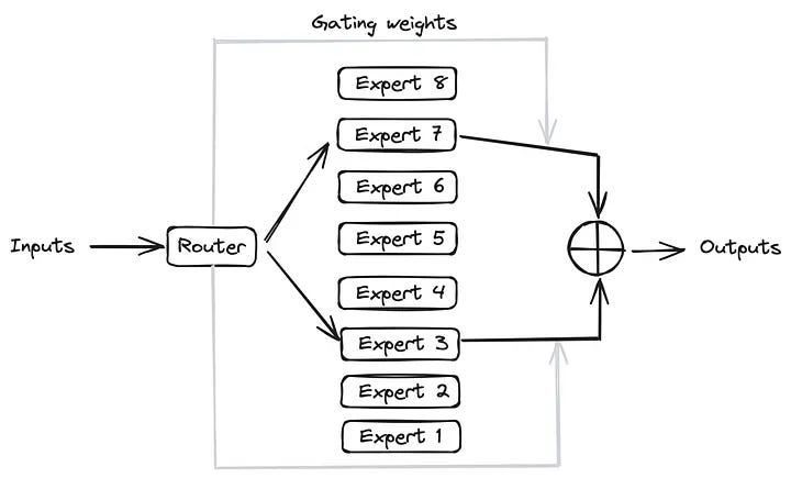
- MOE consists of several sub-networks or "experts" , each trained to handle specific types of data or tasks.
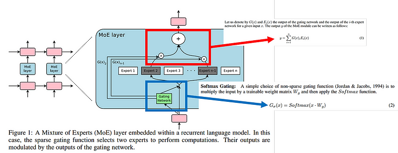
- A gating network determines which expert(s) should process each input , the gating mechanism can use various algorithms to allocate inputs, including softmax-based routing or more sophisticated techniques like Sinkhorn routing for balanced expert utilization.
Routing Mechanisms
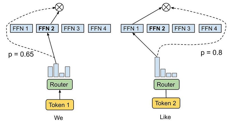
Softmax Token Choice: This router uses a softmax function to compute the affinity between input tokens and experts, ensuring that inputs are directed to the most appropriate experts based on their computed scores.
Sinkhorn Token Choice: This method introduces additional constraints to ensure balanced utilization of experts, which can lead to more efficient training and inference.
Training and Optimization
Gradient Descent: MOE models are typically trained using gradient descent or its variants , each expert learns to handle different aspects of the data, which enhances the overall performance of the model.
Regularization and Auxiliary Losses: Techniques like regularization and auxiliary losses are used to maintain balanced expert usage and prevent overfitting , these methods ensure that all experts are utilized effectively, avoiding the issue of some experts being overburdened while others are underused
MoE Advantages
Scalability: MOE models can handle large-scale machine learning tasks by efficiently distributing the workload across multiple experts.
Specialization: Each expert in an moe model can specialize in different data aspects, resulting in more accurate and precise processing.
Efficiency: Dynamic routing ensures that only the necessary parts of the model are activated, which saves computational resources and reduces processing time.
Challenges
Routing complexity: designing effective routing mechanisms that balance precision and computational efficiency is an ongoing challenge , improvements in routing algorithms are essential for the broader adoption of moe models.
Expert utilization: ensuring balanced and efficient use of experts remains critical , techniques like the sinkhorn token choice are promising, but further enhancements are needed for optimal performance.
Compression and efficiency: while various methods exist to compress moe models, finding the right combination for specific applications is complex , ongoing research in this area aims to optimize these techniques for better model efficiency
Performance Evaluation
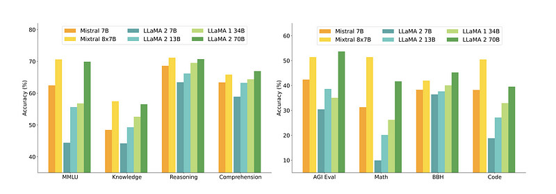
To illustrate the advantages of the moe architecture, we examine the performance of Mixtral, an moe-based model derived from mistral 7b , we compare mixtral's performance against other state-of-the-art models, including gpt-3.5, across multiple tasks such as commonsense reasoning, world knowledge, reading comprehension, math, and code generation.
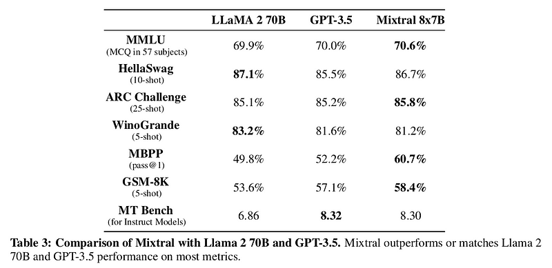
MMLU (Massive Multitask Language Understanding):
- Mixtral: 70.6% accuracy
- Llama 2 70B: 69.9%
- GPT-3.5: 70.2%
Commonsense Reasoning:
- Mixtral on HellaSwag: 84.4%
- Llama 2 70B: 85.4%
- GPT-3.5: 85.1%
Reading Comprehension:
- Mixtral on Natural Questions (NQ): 59.7%
- Llama 2 70B: 56.5%
- GPT-3.5: 58.3%
Math:
- Mixtral on GSM8K: 74.4%
- Llama 2 70B: 69.6%
- GPT-3.5: 72.1%
Code Generation:
- Mixtral on MBPP : 60.7%
- Llama 2 70B: 49.8%
- GPT-3.5: 58.5%
Despite having 5x fewer active parameters during inference, mixtral consistently outperforms or matches the performance of both llama 2 70B and gpt-3.5 on almost all popular benchmarks , this highlights the efficiency and effectiveness of the moe architecture in handling diverse tasks with fewer computational resources.
After learning about the key concepts, cool features, and numerous benefits of the mixture of experts (moe) architecture, it's time to put theory into practice we will dive into coding our own moe model from scratch and train it together , i will guide you through the entire process, explaining the code block by block to ensure a clear and comprehensive understanding.
Code Time
Imports essential dependencies
Import the necessary libraries and modules:
import torch
import time
import torch.nn as nn
import torch.nn.functional as F
from torch.utils.data import DataLoader, Dataset
from datasets import load_dataset
from transformers import AutoTokenizer
Create The DataLoader and Train The Tokenizer
as usual we start this section with the preparation and training of a custom tokenizer, which is a crucial component of our model training pipeline.
First we define a custom dataset class, TextDataset inheriting from pytorch's Dataset , this class is designed to handle our text data efficiently. during initialization it reads the text data from a specified file and prepares it for tokenization , the len method provides the number of text samples, while getitem retrieves a specific text, tokenizes it and prepares it for model input.
class TextDataset(Dataset):
    def __init__(self, file_path, tokenizer, max_length):
        self.tokenizer = tokenizer
        self.max_length = max_length
        with open(file_path, 'r', encoding='utf-8') as f:
            self.texts = f.readlines()

    def __len__(self):
        return len(self.texts)

    def __getitem__(self, idx):
        text = self.texts[idx]
        encoding = self.tokenizer(text, truncation=True,
                                  padding='max_length',
                                  max_length=self.max_length,
                                  return_tensors='pt') # Ensure PyTorch Tensor output

        input_ids = encoding['input_ids'].squeeze()

        # Assuming you want to use the input_ids as labels for language modeling

        labels = input_ids.clone()

        labels[:-1] = input_ids[1:]  # Shift labels
        return input_ids, labels  # Return both input_ids and labels
The get_training_corpus function yields text batches from our cleaned dataset, providing a rich source for training , we train the new tokenizer by iterating over these batches and specifying a vocabulary size.
# Function to get training data
def get_training_corpus():
    dataset = load_dataset("text", data_files={"train": "/content/cleaned_data.txt"})
    for i in range(0, len(dataset["train"]), 1000):
        yield dataset["train"][i : i + 1000]["text"]

# Load the base tokenizer
base_tokenizer = AutoTokenizer.from_pretrained("unsloth/mistral-7b-v0.3-bnb-4bit")

# Train the new tokenizer
new_tokenizer = base_tokenizer.train_new_from_iterator(get_training_corpus(), vocab_size=1000)

# Save the new tokenizer
new_tokenizer.save_pretrained("new_tokenizer")
Once trained we save the new tokenizer and validate its performance by encoding and decoding a sample text , this ensures that the tokenizer effectively handles the specific linguistic features of our dataset , we also address padding, a critical aspect of sequence processing , if the new tokenizer lacks a padding token, we add one, ensuring that all sequences are correctly padded to the maximum length , this step ensures that our tokenizer is fully functional and ready for training our model.
# Test the new tokenizer
test_text = "الهجرة كلمة تسمعها بزاف في بلادي "
encoded = new_tokenizer.encode(test_text)
decoded = new_tokenizer.decode(encoded)

print(f"Encoded: {encoded}")
print(f"Decoded: {decoded}")

# Add padding token if it doesn't exist
if new_tokenizer.pad_token is None:
    new_tokenizer.add_special_tokens({'pad_token': '[PAD]'})

# Ensure pad_token_id is valid
if new_tokenizer.pad_token_id is None or new_tokenizer.pad_token_id >= new_tokenizer.vocab_size:
    new_tokenizer.add_special_tokens({'pad_token': '[PAD]'})
    new_tokenizer.pad_token_id = new_tokenizer.vocab_size - 1  # Use the last valid token ID as padding
Create The model
We sets here the configuration parameters for the model and device, including embedding size, number of attention heads, layers, dropout rate, block size, vocabulary size, number of experts, and top-k for decision-making.
# Configuration parameters
n_embd = 4096
n_head = 32
n_layer = 32
head_size = 128
dropout = 0.1
block_size = 32768
vocab_size = new_tokenizer.vocab_size
num_experts = 8
top_k = 2
# Device configuration
device = 'cuda' if torch.cuda.is_available() else 'cpu'
Attention Head
The Head class implements a single attention head in a self-attention mechanism , it starts by defining linear transformations for the key, query, and value matrices , during the forward pass, it computes the attention weights by applying the dot product of queries and keys, scaled by the square root of the embedding dimension , to ensure causality, it masks future positions using a lower triangular matrix , the attention weights are then softened using softmax and applied to the values to produce the output , dropout is used to improve generalization by randomly setting some weights to zero during training.
class Head(nn.Module):
    def __init__(self, head_size: int):
        super().__init__()
        self.key = nn.Linear(n_embd, head_size, bias=False)
        self.query = nn.Linear(n_embd, head_size, bias=False)
        self.value = nn.Linear(n_embd, head_size, bias=False)
        self.register_buffer('tril', torch.tril(torch.ones(block_size, block_size)))

        self.dropout = nn.Dropout(dropout)

    def forward(self, x: torch.Tensor) -> torch.Tensor:
        B, T, C = x.shape
        k = self.key(x)
        q = self.query(x)
        wei = q @ k.transpose(-2, -1) * C**-0.5
        wei = wei.masked_fill(self.tril[:T, :T] == 0, float('-inf'))
        wei = F.softmax(wei, dim=-1)
        wei = self.dropout(wei)
        v = self.value(x)
        out = wei @ v
        return out
MultiHeadAttention
The MultiHeadAttention class extends the self-attention mechanism by using multiple parallel attention heads , each head independently computes its attention output, allowing the model to focus on different aspects of the input, the outputs from all heads are concatenated and projected back to the original embedding dimension using a linear layer. dropout is applied to the projected output to prevent overfitting.
class MultiHeadAttention(nn.Module):
    def __init__(self, num_heads: int, head_size: int):
        super().__init__()
        self.heads = nn.ModuleList([Head(head_size) for _ in range(num_heads)])
        self.proj = nn.Linear(n_embd, n_embd)
        self.dropout = nn.Dropout(dropout)

    def forward(self, x: torch.Tensor) -> torch.Tensor:
        out = torch.cat([h(x) for h in self.heads], dim=-1)
        out = self.dropout(self.proj(out))
        return out
This architecture enables the model to capture a richer set of dependencies and relationships within the data.
Expert
class Expert(nn.Module):
    def __init__(self, n_embd: int):
        super().__init__()
        self.net = nn.Sequential(
            nn.Linear(n_embd, 4 * n_embd),
            nn.ReLU(),
            nn.Linear(4 * n_embd, n_embd),
            nn.Dropout(dropout),
        )

    def forward(self, x: torch.Tensor) -> torch.Tensor:
        return self.net(x)
The Expert class defines a feedforward neural network, or multilayer perceptron (mlp), which represents an individual expert in the mixture-of-experts model , this network consists of two fully connected layers with a relu activation in between, followed by dropout for regularization , the first layer expands the embedding dimension, while the second layer projects it back to the original size , this setup allows each expert to transform the input embeddings and learn complex patterns within the data.
Router
The Router class manages the allocation of input data to different experts in a mixture-of-experts model, it begins by computing logits that determine how likely it is for each input to be assigned to each expert, and adds noise to these logits to promote robustness and avoid overfitting.
class Router(nn.Module):
    def __init__(self, n_embed: int, num_experts: int, top_k: int):
        super().__init__()
        self.top_k = top_k
        self.topkroute_linear = nn.Linear(n_embed, num_experts)
        self.noise_linear = nn.Linear(n_embed, num_experts)

    def forward(self, mh_output: torch.Tensor):
        logits = self.topkroute_linear(mh_output)
        noise_logits = self.noise_linear(mh_output)
        noise = torch.randn_like(logits) * F.softplus(noise_logits)
        noisy_logits = logits + noise
        top_k_logits, indices = noisy_logits.topk(self.top_k, dim=-1)
        zeros = torch.full_like(noisy_logits, float('-inf'))
        sparse_logits = zeros.scatter(-1, indices, top_k_logits)
        router_output = F.softmax(sparse_logits, dim=-1)
        return router_output, indices
The top_k parameter controls the number of experts to which each input is routed , the forward method calculates the top-k expert logits, which are then converted into a sparse format where only the top-k experts are active , this sparse representation is used to compute the final routing probabilities, which guide how the input data is distributed among the available experts.
MoE Layer
The MoE class orchestrates the routing of inputs through multiple experts in a neural network , during initialization it sets up a Router to decide how inputs are distributed among the experts and creates a list of Expert modules.
class MoE(nn.Module):
    def __init__(self, n_embed: int, num_experts: int, top_k: int):
        super().__init__()
        self.router = Router(n_embed, num_experts, top_k)
        self.experts = nn.ModuleList([Expert(n_embed) for _ in range(num_experts)])
        self.top_k = top_k

    def forward(self, x: torch.Tensor) -> torch.Tensor:
        gating_output, indices = self.router(x)
        final_output = torch.zeros_like(x)

        flat_x = x.view(-1, x.size(-1))
        flat_gating_output = gating_output.view(-1, gating_output.size(-1))

        for i, expert in enumerate(self.experts):
            expert_mask = (indices == i).any(dim=-1)
            flat_mask = expert_mask.view(-1)

            if flat_mask.any():
                expert_input = flat_x[flat_mask]
                expert_output = expert(expert_input)
                gating_scores = flat_gating_output[flat_mask, i].unsqueeze(1)
                weighted_output = expert_output * gating_scores
                final_output[expert_mask] += weighted_output.squeeze(1)

        return final_output
In the forward method the Router generates routing probabilities for the inputs determining which experts should handle each input , it then iterates through each expert, applying a mask to select inputs assigned to that expert, and computes the expert's output.
This output is weighted by the routing scores to adjust its contribution , the results from all experts are aggregated to produce the final output, ensuring that each input is processed by its assigned experts with appropriate weighting.
MoE Block
The Block class implements a mixture of experts transformer block, combining self-attention mechanisms with a mixture of experts, it initializes with a multi-head self-attention layer and an moe layer, each tailored to the embedding size and the number of experts.
class Block(nn.Module):
    def __init__(self, n_embed: int, n_head: int, num_experts: int, top_k: int):
        super().__init__()
        head_size = n_embed // n_head
        self.sa = MultiHeadAttention(n_head, head_size)
        self.smoe = MoE(n_embed, num_experts, top_k)
        self.ln1 = nn.LayerNorm(n_embed)
        self.ln2 = nn.LayerNorm(n_embed)

    def forward(self, x: torch.Tensor) -> torch.Tensor:
        x = x + self.sa(self.ln1(x))
        x = x + self.smoe(self.ln2(x))
        return x
The forward pass begins by applying layer normalization to the input, passing it through the multi-head attention mechanism, and then adding the result to the original input for residual connection, this processed input is then normalized again and fed into the moe layer, which incorporates multiple expert networks..
The output from the moe layer is added to the previous result, completing the residual connection , this approach ensures that the block leverages both attention mechanisms and expert networks to enhance its representation power.
MoE Transformer
The MOELanguageModel class defines a sophisticated language model that integrates mixture of experts (moe) with transformer architecture , it begins with embedding layers for token and positional information, converting input indices into dense representations and incorporating position-based embeddings to capture sequence order , the model processes these embeddings through a series of transformer blocks, each equipped with self-attention and moe layers , after passing through these blocks, the output is normalized and projected into the vocabulary space using a linear layer to produce logits.
class MOELanguageModel(nn.Module):
    def __init__(self):
        super().__init__()
        self.token_embedding_table = nn.Embedding(vocab_size, n_embd)
        self.position_embedding_table = nn.Embedding(block_size, n_embd)
        self.blocks = nn.Sequential(
            *[Block(n_embd, n_head, num_experts, top_k) for _ in range(n_layer)]
        )
        self.ln_f = nn.LayerNorm(n_embd)
        self.lm_head = nn.Linear(n_embd, vocab_size)

    def forward(self, idx: torch.Tensor, targets: torch.Tensor = None):
        B, T = idx.shape
        tok_emb = self.token_embedding_table(idx)  # (B, T, n_embd)
        pos_emb = self.position_embedding_table(torch.arange(T, device=device))  # (T, n_embd)
        x = tok_emb + pos_emb  # (B, T, n_embd)
        x = self.blocks(x)  # (B, T, n_embd)
        x = self.ln_f(x)  # (B, T, n_embd)
        logits = self.lm_head(x)  # (B, T, vocab_size)

        loss = None
        if targets is not None:
            B, T, C = logits.shape
            logits = logits.view(B * T, C)
            targets = targets.view(B * T)
            loss = F.cross_entropy(logits, targets)

        return logits, loss

    def generate(self, idx: torch.Tensor, max_new_tokens: int) -> torch.Tensor:
        for _ in range(max_new_tokens):
            idx_cond = idx[:, -block_size:]
            logits, _ = self(idx_cond)
            logits = logits[:, -1, :]
            probs = F.softmax(logits, dim=-1)
            idx_next = torch.multinomial(probs, num_samples=1)
            idx = torch.cat((idx, idx_next), dim=1)
        return idx
So during training if target labels are provided, the model computes the cross-entropy loss to measure the prediction error against the targets ,for text generation the model predicts one token at a time ,it uses the last block_size tokens from the current sequence to generate the next token based on probability distributions derived from the logits , this process iteratively extends the sequence until the desired length is reached (32k in our case).
model = MOELanguageModel().to(device)
This line initializes an instance of the MOELanguageModel class and moves it to the specified device (e.g., gpu or cpu) for training or inference , this setup ensures that the model's computations and parameters are compatible with the hardware on which you are running your code , by placing the model on the appropriate device, you optimize performance and enable efficient processing.
Setup The Trainer
The Train function is designed to handle the training of the MOELanguageModel, it begins by setting up the model on the appropriate device, either gpu or cpu, and activating training mode , inside the main training loop, the function iterates over batches of training data, performing a forward pass to compute predictions and loss , it then executes backpropagation to calculate gradients and applies gradient clipping to prevent issues with exploding gradients.
def train(model: SMoELanguageModel,
          train_data: DataLoader,
          val_data: DataLoader,
          optimizer: torch.optim.Optimizer,
          total_steps: int = 10000,
          device: str = 'cuda' if torch.cuda.is_available() else 'cpu',
          clip_grad_norm: float = 1.0,
          lr_scheduler=None,
          eval_interval: int = 1000,
          save_path: str = "MOE_darija.pt"):

    model = model.to(device)
    model.train()

    print("Training...")
    step = 0
    total_loss = 0.0
    start_time = time.time()

    while step < total_steps:
        for batch in train_data:
            input_ids, labels = batch
            input_ids, labels = input_ids.to(device), labels.to(device)

            # Forward pass
            optimizer.zero_grad()
            logits, loss = model(input_ids, labels)

            # Backward pass
            loss.backward()

            # Clip gradients
            torch.nn.utils.clip_grad_norm_(model.parameters(), clip_grad_norm)

            # Update weights
            optimizer.step()

            if lr_scheduler is not None:
                lr_scheduler.step(loss.detach().item())

            total_loss += loss.item()
            step += 1

            # Print step-wise loss and elapsed time periodically
            if step % eval_interval == 0:
                avg_loss = total_loss / eval_interval
                elapsed_time = time.time() - start_time
                print(f"Step {step}/{total_steps} | Average loss: {avg_loss:.4f} | Elapsed time: {elapsed_time:.2f}s")
                total_loss = 0.0
                start_time = time.time()

                # Evaluation Phase
                model.eval()
                eval_loss = 0
                with torch.no_grad():
                    for val_batch in val_data:
                        input_ids, labels = val_batch
                        input_ids, labels = input_ids.to(device), labels.to(device)
                        logits, loss = model(input_ids, labels)
                        eval_loss += loss.item()

                avg_eval_loss = eval_loss / len(val_data)
                print(f"Step {step}, Evaluation Loss: {avg_eval_loss:.4f}")
                model.train()

            # Stop if total steps reached
            if step >= total_steps:
                break

        # Early stop if steps are already reached within epoch
        if step >= total_steps:
            break

    torch.save(model.state_dict(), save_path)
    print("Training complete!")
The optimizer updates the model's weights based on these gradients, and if a learning rate scheduler is provided, it adjusts the learning rate accordingly , periodically the function logs the average loss and elapsed time to track progress , additionally at specified intervals the model is evaluated on a validation dataset to gauge performance and ensure it is not overfitting. Once the total number of training steps is reached, the function saves the model's state dictionary to a file and prints a completion message , this comprehensive training process ensures that the model is effectively trained and validated throughout its learning phase.
Create the Optimizer and Learning rate Scheduler
The optimizer and learning rate scheduler are configured for training the model , the AdamW optimizer is chosen for its efficiency in training deep learning models by using adaptive learning rates for each parameter.
optimizer = torch.optim.AdamW(model.parameters(), lr=1e-4)
lr_scheduler = torch.optim.lr_scheduler.ReduceLROnPlateau(optimizer, 'min', patience=3)
It's initialized a learning rate of 1e-4 which is a common choice for fine-tuning deep models , also a learning rate scheduler ReduceLROnPlateau, is used to adjust the learning rate based on the performance of the model , this scheduler monitors the validation loss, and if it plateaus ( stops improving ) for a specified number of training steps, it reduces the learning rate.
The patience parameter is set to 3 meaning the learning rate will only be reduced after three consecutive steps without improvement in the validation loss , this approach helps in refining the training process, allowing the model to converge more effectively and avoid overfitting.
Create Train and valid Datasets
The training and validation datasets are prepared and loaded for model training , a custom TextDataset class is used to handle the text data, which is tokenized and converted into tensors compatible with the model , the TextDataset class is initialized with the path to the cleaned training data file, the newly trained tokenizer and a maximum sequence length of 512 tokens (you can make it bigger till 32k) similarly the validation dataset is set up with a separate validation file.
train_dataset = TextDataset('/content/cleaned_data.txt',
                            new_tokenizer,
                            max_length=512)
train_loader = DataLoader(train_dataset,
                          batch_size=4,
                          shuffle=False)

val_dataset = TextDataset('/content/validation.txt',
                            new_tokenizer,
                            max_length=512)
val_loader = DataLoader(val_dataset,
                          batch_size=4,
                          shuffle=False)
The DataLoader is then used to manage batching and shuffling of the data , for both the training and validation datasets, the DataLoader is configured with a batch size of 4, which means each batch will contain 4 samples , shuffling is disabled for both loaders, ensuring that the order of samples remains consistent, which can be particularly useful during validation to assess the model's performance on the data in a predictable manner.
Kick off the training :
train(model,
      train_loader,
      val_loader,
      optimizer)
Inference
max_length = 30
num_return_sequences = 10

# Encode the input text
tokens = new_tokenizer.encode("راك ")
tokens = torch.tensor(tokens, dtype=torch.long)
tokens = tokens.unsqueeze(0).repeat(num_return_sequences, 1)

# Generate sequences
ids = model.generate(tokens,max_length)

# Print the generated text
for i in range(num_return_sequences):
    decoded = new_tokenizer.decode(ids[i], skip_special_tokens=True)
    print(">", decoded)
The max_length parameter is set to 30 and num_return_sequences is set to 10, indicating that the model should generate 10 sequences of text, each up to 30 tokens long , the input text راك is first encoded into token ids using the new_tokenizer, then converted to a pytorch tensor and repeated to match the desired number of sequences , the model.generate method is then used to produce the sequences based on the input tokens , finally each generated sequence is decoded back into text and printed out , this process showcases the model's ability to generate multiple diverse outputs from a single input prompt, highlighting its potential for creative text generation.