LLaMa2 from Scratch
Llama 2 🦙
Llama 2, developed by Meta AI, is an open-source family of large language models (LLMs) that includes various models ranging from 7 billion to 70 billion parameters ,these models are designed to generate text and can be fine-tuned for specific tasks, making them versatile for various natural language processing (NLP) applications , the Llama 2 models are an evolution of the original Llama models, offering improvements in performance, efficiency, and usability.

Model Architecture
Llama 2 uses a transformer architecture (decoder-only) optimized for auto-regressive language modeling. key architectural features include:
Pre-Normalization
Pre-normalization in transformers refers to applying layer normalization before the main operations within each transformer block, rather than after. This technique stabilizes training by ensuring that the input to each sub-layer (e.g., attention and feed-forward) is well-conditioned.
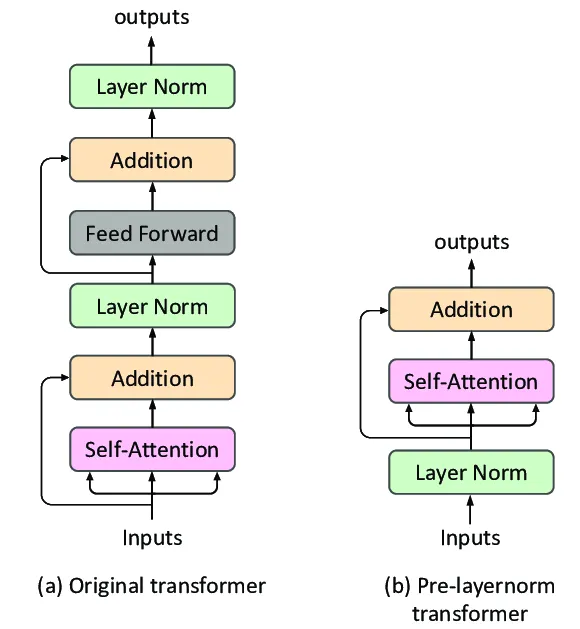
Pre-normalization addresses the issue of exploding or vanishing gradients, leading to more stable and faster convergence during training, by normalizing inputs before any transformation, pre-normalization allows the model to maintain more consistent gradient magnitudes, which is particularly beneficial in training very deep transformer architectures
SwiGLU Activation Function
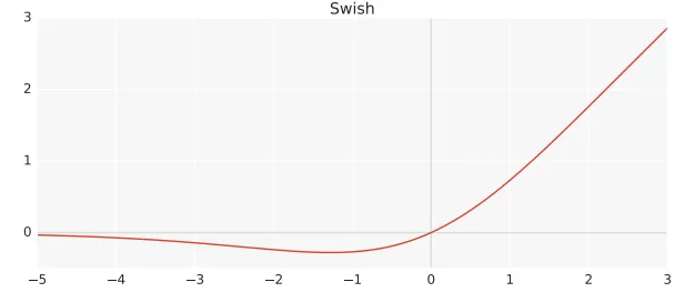
The SwiGLU (Swish-Gated Linear Unit) activation function is a variant of the popular GLU (Gated Linear Unit) family, designed to improve the performance of neural networks by combining Swish and GLU.
Swish is defined as :
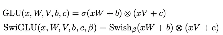
where beta β is a trainable parameter, and GLU uses a gating mechanism to control the flow of information, SwiGLU applies the Swish activation to the gating mechanism, creating a smoother and more flexible gating function.
This results in better gradient flow during training and improved model performance, particularly in deep networks
Rotary Positional Embeddings
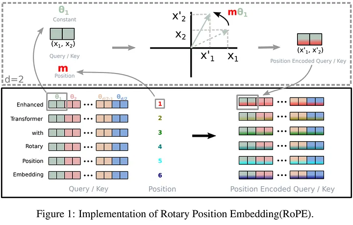
Rotary Positional Embeddings (RoPE) offer an innovative method to incorporate positional information in transformer models, encoding absolute positional information through rotation matrices, this technique naturally introduces relative position dependency within the self-attention mechanism,traditional positional embeddings add positional encodings to token embeddings, while RoPE modifies the embeddings through rotations, mixing pairs of coordinates.
The rotation matrix ensures that the relative position information decays as the distance between tokens increases, reflecting the intuitive idea that tokens further apart have weaker connections. This method is computationally efficient and scales well with sequence length, enhancing model performance across various tasks
Grouped-Query Attention (GQA)
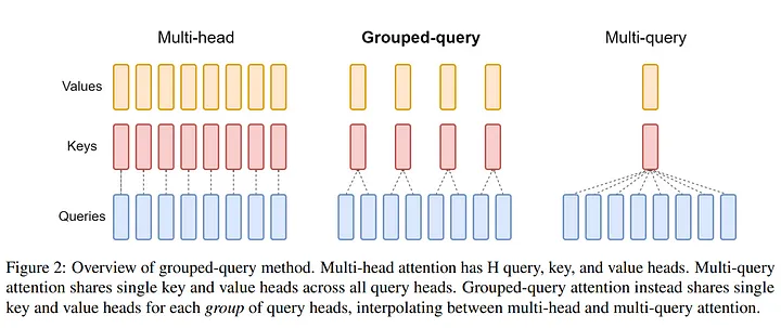
Grouped-Query Attention (GQA) is an advanced mechanism that enhances the efficiency of self-attention in transformers by grouping multiple queries together, instead of computing attention scores individually for each query, GQA processes groups of queries simultaneously, reducing the computational complexity.
This approach improves memory usage and speeds up training and inference without compromising model performance. GQA is particularly useful in large-scale models where traditional self-attention mechanisms become computationally expensive and memory-intensive. By optimizing the way queries are handled, GQA enables more scalable and efficient transformer models.
Code Time
Data Preparation
Before diving into the code, it’s important to note that the dataset we’re using here is not fully cleaned. if you have access to a better-quality dataset, it’s advisable to use that instead. for this guide, we’re working with the v1 split, which contains almost 170k rows of raw data, mainly for testing and experimentation purposes.
import pandas as pd

splits = {'v1': 'data/v1-00000-of-00001.parquet'}
df = pd.read_parquet("hf://datasets/ayoubkirouane/Algerian-Darija/" + splits["v1"])
text = df['Text'].to_list()

with open('cleaned_data.txt', 'w') as f:
  f.write('\n'.join(text))
To prepare our dataset for further use, we need to read the raw data and save it in a more manageable format.
First, we import the pandas library, which is a powerful tool for data manipulation and analysis.
Next, we specify the path to our dataset split, which in this case is labeled v1. We read the Parquet file from Hugging Face into a DataFrame, a tabular data structure provided by pandas.
After loading the data, we extract the text from the Text column and convert it into a list. This list contains all the text entries from our dataset, which we will then write to a text file.
Finally, we open a file called cleaned_data.txt in write mode and save the extracted text data to this file, with each text entry separated by a newline. This step creates a plain text file that we can use for further processing in our project.
Create Llama Tokenizer and train it
To build a tokenizer specifically for our Algerian Darija dataset, we follow these steps to create and test a new tokenizer tailored to our text data.
First, we import the necessary libraries: LlamaTokenizerFast from transformers for managing the tokenizer and load_dataset from datasets for loading our data.
We start by defining a function called get_training_corpus(). this function loads our cleaned data from a text file and splits it into chunks of 1000 text samples at a time. this chunked approach is useful for efficiently processing the data and feeding it to the tokenizer.
Next, we initialize a base tokenizer using the LlamaTokenizerFast class from a pre-trained model. This tokenizer serves as our starting point for building a new tokenizer.
from transformers import LlamaTokenizerFast
from datasets import load_dataset

# Function to get training data
def get_training_corpus():
    dataset = load_dataset("text", data_files={"train": "cleaned_data.txt"})
    for i in range(0, len(dataset["train"]), 1000):
        yield dataset["train"][i : i + 1000]["text"]

# Initialize the base tokenizer
base_tokenizer = LlamaTokenizerFast.from_pretrained("hf-internal-testing/llama-tokenizer")

# Train the new tokenizer
new_tokenizer = base_tokenizer.train_new_from_iterator(get_training_corpus(), vocab_size=1000)

# Save the new tokenizer
new_tokenizer.save_pretrained("darija_tokenizer")

# Test the new tokenizer
test_text = "الهجرة كلمة تسمعها بزاف"
encoded = new_tokenizer.encode(test_text)
decoded = new_tokenizer.decode(encoded)

print(f"Encoded: {encoded}")
print(f"Decoded: {decoded}")
With the base tokenizer ready, we proceed to train our new tokenizer. we use the train_new_from_iterator() method, feeding it the text chunks generated by our get_training_corpus() function and setting a vocabulary size of 1000. This step creates a tokenizer that is better suited for the specific vocabulary and text patterns found in Algerian Darija.
After training, we save the new tokenizer to a specified directory using the save_pretrained() method. this saved tokenizer can be used later for tokenizing text data in our model training process.
Finally, we test our new tokenizer by encoding and decoding a sample text in Algerian Darija. We print out the encoded token IDs and the decoded text to verify that our tokenizer processes the text as expected.
Setting Up Model Configuration and Training Parameters
Here we define two key classes that will help us configure and train our Llama2 model effectively.
First, we set up the ModelArgs class, which specifies the fundamental architecture of our model. This includes everything from the number of layers to the size of the hidden dimensions. These settings are crucial for shaping how our model will learn and perform on the Algerian Darija text.
class ModelArgs:
    def __init__(self, dim=4096,
                 n_layers=32,
                 n_heads=32,
                 n_kv_heads=None,
                 vocab_size=-1,
                 multiple_of=256,
                 ffn_dim_multiplier=None,
                 norm_eps=1e-5,
                 mode='train',
                 batch_size=32,
                 max_seq_length=32,
                 device='cuda' if torch.cuda.is_available() else 'cpu', pad_token_id=None):
        self.dim = dim
        self.n_layers = n_layers
        self.n_heads = n_heads
        self.n_kv_heads = n_kv_heads
        self.vocab_size = vocab_size
        self.multiple_of = multiple_of
        self.ffn_dim_multiplier = ffn_dim_multiplier
        self.norm_eps = norm_eps
        self.mode = mode
        self.batch_size = batch_size
        self.max_seq_length = max_seq_length
        self.device = device
        self.pad_token_id = pad_token_id

class TrainArgs(ModelArgs):
    def __init__(self, n_epochs=10,
                 log_interval=12,
                 eval_iters=200,
                 lr=3e-4,
                 warmup_steps=4000,
                 **kwargs):
        super().__init__(**kwargs)
        self.n_epochs = n_epochs
        self.log_interval = log_interval
        self.eval_iters = eval_iters
        self.lr = lr
        self.warmup_steps = warmup_steps
Next, the TrainArgs class builds on this setup by adding parameters specific to the training process itself. We cover things like the number of training epochs, learning rate, and directories for saving and loading models. These settings help manage the training workflow and ensure we can track progress and make improvements.
Implementing RMSNorm for Normalization
In this section, we implement the RMSNorm class, a custom normalization layer used in our model. RMSNorm stands for “Root Mean Square Layer Normalization” and it is a variant of the traditional layer normalization.
we start by defining the RMSNorm class, inheriting from nn.Module. this class is designed to perform normalization on the model’s activations.
in the forward method, we compute the RMS of the input tensor along the last dimension. the tensor is then scaled by self.scale and divided by the square root of the RMS value plus a small constant eps for numerical stability. this approach helps stabilize training and improve model performance.
class RMSNorm(nn.Module):
    def __init__(self, dim, eps=1e-5):
        super().__init__()
        self.eps = eps
        self.scale = nn.Parameter(torch.ones(dim))

    def forward(self, x):
        norm = x.norm(2, dim=-1, keepdim=True)
        return self.scale * x / torch.sqrt(norm ** 2 + self.eps)
Implementing SwiGLU Activation Function
In the architecture section, we explored the role of SwiGLU as a crucial component of our model.
class SwiGLU(nn.Module):
    def __init__(self, dim_in, dim_out):
        super().__init__()
        self.linear1 = nn.Linear(dim_in, dim_out)
        self.linear2 = nn.Linear(dim_in, dim_out)

    def forward(self, x):
        return F.silu(self.linear1(x)) * self.linear2(x)
The SwiGLU class is defined with two linear layers. In the forward method, the input tensor x is first passed through the first linear layer and then activated using the Swish function. this result is then multiplied element-wise with the output of the second linear layer, which helps to regulate the flow of information through the network.
Implementing Rotary Embedding
In the architecture section, we discussed the importance of Rotary Embedding for our model. now let’s delve into the code for this component.
class RotaryEmbedding(nn.Module):
    def __init__(self, dim):
        super().__init__()
        inv_freq = 1.0 / (10000 ** (torch.arange(0, dim, 2).float() / dim))
        self.register_buffer('inv_freq', inv_freq)

    def forward(self, seq_len, device):
        t = torch.arange(seq_len, device=device).type_as(self.inv_freq)
        freqs = torch.einsum('i,j->ij', t, self.inv_freq)
        emb = torch.cat((freqs, freqs), dim=-1)
        return emb
The RotaryEmbedding class generates the rotary positional embeddings used to encode position information in the input sequences. this approach introduces a way to handle positional information in a more sophisticated manner than traditional methods.
Grouped Query Attention Mechanism
The GroupedQueryAttention class implements a variant of the attention mechanism that processes queries, keys, and values in separate groups. This approach divides the attention mechanism into multiple heads and groups, allowing the model to focus on different aspects of the data simultaneously.
class GroupedQueryAttention(nn.Module):
    def __init__(self, dim, n_heads, n_kv_heads):
        super().__init__()
        self.n_heads = n_heads
        self.n_kv_heads = n_kv_heads
        self.query = nn.Linear(dim, dim)
        self.key = nn.Linear(dim, dim)
        self.value = nn.Linear(dim, dim)
        self.out = nn.Linear(dim, dim)

    def forward(self, x):
        batch_size, seq_length, dim = x.size()
        q = self.query(x).view(batch_size, seq_length, self.n_heads, dim // self.n_heads)
        k = self.key(x).view(batch_size, seq_length, self.n_kv_heads, dim // self.n_kv_heads)
        v = self.value(x).view(batch_size, seq_length, self.n_kv_heads, dim // self.n_kv_heads)

        scores = torch.einsum('bhqd, bhkd -> bhqk', q, k) / math.sqrt(dim // self.n_heads)
        attn = torch.nn.functional.softmax(scores, dim=-1)
        context = torch.einsum('bhqk, bhvd -> bhqd', attn, v)
        context = context.contiguous().view(batch_size, seq_length, dim)
        return self.out(context)
In this implementation, GroupedQueryAttention handles the creation of queries, keys, and values, computes attention scores, and applies these scores to extract contextual information from the inputs.
Queries, Keys, and Values: the class initializes linear layers for transforming input data into queries, keys, and values.
Attention Calculation: it computes attention scores by comparing queries and keys and then applies the softmax function to get attention weights.
Context Extraction: it uses these weights to combine values and produce the final output.
Transformer Block
The TransformerBlock class encapsulates a fundamental building block of the Transformer architecture, designed to perform multi-head attention and feed-forward processing while integrating additional features like Rotary Embeddings.
class TransformerBlock(nn.Module):
    def __init__(self, args):
        super().__init__()
        self.attn = GroupedQueryAttention(args.dim, args.n_heads, args.n_kv_heads)
        self.norm1 = RMSNorm(args.dim, args.norm_eps)
        self.norm2 = RMSNorm(args.dim, args.norm_eps)
        self.mlp = nn.Sequential(
            nn.Linear(args.dim, args.ffn_dim_multiplier * args.dim),
            SwiGLU(args.ffn_dim_multiplier * args.dim, args.dim)
        )
        self.rotary_emb = RotaryEmbedding(args.dim)

    def forward(self, x):
        seq_len, device = x.shape[1], x.device
        rotary_emb = self.rotary_emb(seq_len, device)  # Should match x.shape[2]
        x = x + rotary_emb

        attn_out = self.attn(self.norm1(x))
        x = x + attn_out

        mlp_out = self.mlp(self.norm2(x))
        x = x + mlp_out

        return x
Attention Mechanism: the GroupedQueryAttention layer applies multi-head attention using separate query, key, and value groups to capture complex relationships in the data.
Normalization: two RMSNorm layers are used to stabilize training by normalizing the outputs of the attention and feed-forward layers.
Feed-Forward Network: A multi-layer perceptron (MLP) with a SwiGLU activation function transforms the data from one representation to another, enhancing the model’s capacity to learn complex patterns.
Rotary Embeddings: RotaryEmbedding adds positional encodings to the input data, helping the model understand the order of tokens.
In the forward method:
- Add Rotary Embeddings: positional encodings are added to the input.
- Attention Operation : multi-head attention is performed, and the result is added to the input (residual connection).
- Feed-Forward Processing: the data is passed through the feed-forward network, and the result is added to the input (another residual connection).
The Transformer Class
In this section we define the Transformer class, which integrates the key components of the Llama 2 Transformer to process and generate sequences.
class Transformer(nn.Module):
    def __init__(self, args):
        super().__init__()
        self.token_emb = nn.Embedding(args.vocab_size, args.dim, padding_idx=args.pad_token_id)
        self.blocks = nn.ModuleList([TransformerBlock(args) for _ in range(args.n_layers)])
        self.norm = RMSNorm(args.dim, args.norm_eps)
        self.head = nn.Linear(args.dim, args.vocab_size, bias=False)

    def forward(self, x):
        x = self.token_emb(x)
        for block in self.blocks:
            x = block(x)
        x = self.norm(x)
        logits = self.head(x)
        return logits
Token Embeddings: the nn.Embedding layer transforms input token indices into dense vectors of a specified dimension. This layer learns the representations of tokens, with an option for padding tokens if needed.
Transformer Blocks: a ModuleList contains multiple TransformerBlock instances, each performing self-attention and feed-forward operations. The number of blocks corresponds to the model’s depth, and they are applied sequentially to process the token embeddings.
Normalization: RMSNorm is applied to the output of the last Transformer block. This normalization step stabilizes the learning process and helps the model converge.
Output Head: a Linear layer projects the model’s output from the hidden dimension to the vocabulary size, generating logits for each token in the vocabulary. This layer does not have a bias term, as it is typically not required for language modeling tasks.
In the forward method:
- Token Embedding Lookup: the input token indices are converted into dense vectors. Pass Through Transformer Blocks: the token embeddings are processed through a series of transformer blocks.
- Apply Normalization: the output from the final transformer block is normalized.
- Generate Logits: the final dense layer produces logits for each token, which can be used for predictions in tasks such as language modeling.
The train_model Function
This function is responsible for training the Transformer model on the given data. It includes the training loop, evaluation phase, and also handles learning rate scheduling and loss computation.
# Train_model function
def train_model(model, train_loader, eval_loader, train_args, tokenizer):
    model = model.to(train_args.device)
    optimizer = torch.optim.AdamW(model.parameters(), lr=train_args.lr)
    scheduler = torch.optim.lr_scheduler.LambdaLR(optimizer, lr_lambda=lambda step: min(1.0, step / train_args.warmup_steps))

    for epoch in range(train_args.n_epochs):
        model.train()
        for step, batch in enumerate(train_loader):
                input_ids, labels = batch
                input_ids, labels = input_ids.to(train_args.device), labels.to(train_args.device)

                outputs= model(input_ids)
                loss_fn = nn.CrossEntropyLoss()
                loss = loss_fn(outputs.view(-1, tokenizer.vocab_size), labels.view(-1))
                loss.backward()
                optimizer.step()
                scheduler.step()
                optimizer.zero_grad()
                if step % train_args.log_interval == 0:
                    print(f"Epoch: {epoch}, Step: {step}, Loss: {loss.item()}")
        model.eval()
        eval_loss = 0
        with torch.no_grad():
            for step, batch in enumerate(eval_loader):
                input_ids, labels = batch

                input_ids, labels = input_ids.to(train_args.device), labels.to(train_args.device)
                outputs= model(input_ids)

                loss_fn = nn.CrossEntropyLoss()
                loss = loss_fn(outputs.view(-1, tokenizer.vocab_size), labels.view(-1))
                eval_loss += loss.item()
        print(f"Epoch: {epoch}, Evaluation Loss: {eval_loss / len(eval_loader)}")

        # Save the trained model
        model_save_path = "llama2_darija"
        torch.save(model.state_dict(), model_save_path)
        print(f"Model saved to {model_save_path}")
Move Model to Device: the model is moved to the appropriate computing device (CPU or GPU) as specified by the train_args.device.
Optimizer and Scheduler: AdamW optimizer is used for updating the model’s parameters, with a learning rate scheduler that adjusts the learning rate based on the number of warmup steps.
Training Loop: for each epoch, the model processes batches of training data. The loss is computed using cross_entropy, which compares the model’s predictions against the true token indices. the optimizer updates the model parameters based on the loss, and the learning rate scheduler steps forward.
Logging: training progress is logged at intervals specified by train_args.log_interval, showing the current epoch, step, and loss value.
Evaluation Phase: after each epoch, the model’s performance is evaluated on the validation data, the evaluation loss is computed in a no-gradient context to prevent unnecessary computations.
Exception Handling: if an error occurs during training, details about the error are printed, including the shape and value range of the last batch processed.
Data loader
This class is a custom Dataset implementation for loading and tokenizing text data. It is designed to be used with PyTorch’s DataLoader to handle text data for model training or evaluation.
class TextDataset(Dataset):
    def __init__(self, file_path, tokenizer, max_length):
        self.tokenizer = tokenizer
        self.max_length = max_length
        with open(file_path, 'r', encoding='utf-8') as f:
            self.texts = f.readlines()

    def __len__(self):
        return len(self.texts)

    def __getitem__(self, idx):
        text = self.texts[idx]
        encoding = self.tokenizer(text, truncation=True,
                                  padding='max_length',
                                  max_length=self.max_length,
                                  return_tensors='pt') # Ensure PyTorch Tensor output

        input_ids = encoding['input_ids'].squeeze()

        # Assuming you want to use the input_ids as labels for language modeling

        labels = input_ids.clone()

        labels[:-1] = input_ids[1:]  # Shift labels
        return input_ids, labels  # Return both input_ids and labels
Adding and Validating the Padding Token
In the following steps, we ensure that the tokenizer has a valid padding token for handling sequences of varying lengths:
# Add padding token if it doesn't exist
if new_tokenizer.pad_token is None:
    new_tokenizer.add_special_tokens({'pad_token': '[PAD]'})

# Ensure pad_token_id is valid
if new_tokenizer.pad_token_id is None or new_tokenizer.pad_token_id >= new_tokenizer.vocab_size:
    new_tokenizer.add_special_tokens({'pad_token': '[PAD]'})
    new_tokenizer.pad_token_id = new_tokenizer.vocab_size - 1  # Use the last valid token ID as padding
Add Padding Token: We check if a padding token is already defined in the tokenizer. If not, we add one with the identifier [PAD]. This token is essential for making all sequences in the dataset the same length during training.
Validate Padding Token ID: After adding the padding token, we confirm that its ID is valid. If the pad_token_id is not set correctly or exceeds the vocabulary size, we fix it by setting the pad_token_id to the last token ID in the vocabulary. This adjustment ensures that padding operations work as expected.
Creating the Dataset and Data Loaders
to get our model ready for training, we need to prepare the dataset and set up data loaders. this step involves converting raw text data into a format that the model can process and organizing it into batches for training.
# Create dataset and dataloaders
train_dataset = TextDataset('cleaned_data.txt', new_tokenizer, max_length=512)
train_loader = DataLoader(train_dataset, batch_size=32, shuffle=False)

# here you need validation data you can create your our or split your cleaned_data into train and eval
eval_dataset = TextDataset('validation_data.txt', new_tokenizer, max_length=512)
eval_loader = DataLoader(eval_dataset, batch_size=32, shuffle=False)
with the data prepared, it’s time to configure and initialize our llama2 model. this involves setting up the model’s hyperparameters and creating an instance of the Transformer class.
we start by defining the ModelArgs class with the necessary parameters for our model. this includes the dimensions, number of layers, and other configuration details specific to our model architecture.
Initialize llama2 model
model_args = ModelArgs(
    dim=4096,
    n_layers=32,
    n_heads=32,
    n_kv_heads=256,
    vocab_size=new_tokenizer.vocab_size,
    ffn_dim_multiplier=4,
    norm_eps=1e-5,
    batch_size=32,
    max_seq_length=512,
    device='cuda' if torch.cuda.is_available() else 'cpu',
    pad_token_id=new_tokenizer.pad_token_id  # Ensure this value is within the vocabulary size
)
# Initialize model
model = Transformer(model_args)
n_layers: the number of transformer layers in the model.n_heads: the number of attention heads used in the multi-head attention mechanism.dim: the dimensionality of the model’s hidden states.n_kv_heads: the number of key and value heads for attention.vocab_size: the size of the vocabulary, determined by the tokenizer we trained.ffn_dim_multiplier: multiplier for the feed-forward network dimension.norm_eps: epsilon value for layer normalization.batch_size: the number of samples per batch during training.max_seq_length: the maximum sequence length for the input texts.device: the hardware device for computation (cuda for GPU or cpu for CPU).pad_token_id: the token ID used for padding sequences.
Initializing Training Arguments and Starting Training
Next, we set up the training configuration with the TrainArgs class ,This step involves specifying the number of epochs, learning rate, and other training parameter , once the configuration is complete, the train_model function is called to begin the training process.
# Initialize training arguments
train_args = TrainArgs(
    n_epochs=10,      # Number of epochs to train the model
    log_interval=12,  # How often to log the training progress
    lr=3e-4,          # Learning rate for the optimizer
    warmup_steps=4000,# Number of warmup steps for the learning rate scheduler
    device='cuda' if torch.cuda.is_available() else 'cpu',# Compute device
    vocab_size=new_tokenizer.vocab_size # Size of the model's vocabulary
)
# Train the model
train_model(model, train_loader, eval_loader, train_args, new_tokenizer)
Inference Time
In this section, we set up the inference process for generating text sequences.
We first specify the maximum length for the generated text and the number of sequences to produce.
The input text "وحد نهار" is tokenized into IDs, and we prepare these tokens for processing by adding a batch dimension and moving them to the appropriate device (GPU or CPU).
# Set the maximum length of the generated text to 30
max_length = 30
device='cuda' if torch.cuda.is_available() else 'cpu'
# Set the number of sequences to generate to 5
num_return_sequences = 5

# Tokenize the input text "وحد نهار" using the new_tokenizer and convert it to a PyTorch tensor
tokens = new_tokenizer.encode("وحد نهار")
tokens = torch.tensor(tokens, dtype=torch.long)

# Add a batch dimension to the input tensor and repeat it num_return_sequences times to generate multiple sequences
tokens = tokens.unsqueeze(0).repeat(num_return_sequences, 1)

# Move the input tensor to the device (GPU if available, otherwise CPU)
x = tokens.to(device)

while x.size(1) < max_length:
    # forward the model to get the logits
    with torch.no_grad():
        outputs = model(x) # (B, T, vocab_size)
        # take the logits at the last position
        logits = outputs[0] if isinstance(outputs, tuple) else outputs
        logits = logits[:, -1, :] # (B, vocab_size)
        # get the probabilities
        probs = F.softmax(logits, dim=-1)
        # topk_probs here becomes (5, 50), topk_indices is (5, 50)
        topk_probs, topk_indices = torch.topk(probs, 50, dim=-1)
        # select a token from the top-k probabilities
        # note: multinomial does not demand the input to sum to 1
        ix = torch.multinomial(topk_probs, 1) # (B, 1)
        # gather the corresponding indices
        xcol = torch.gather(topk_indices, -1, ix) # (B, 1)
        # append to the sequence
        x = torch.cat((x, xcol), dim=1)

# print the generated text
for i in range(num_return_sequences):
    tokens = x[i, :max_length].tolist()
    decoded = new_tokenizer.decode(tokens)
    print(">", decoded)
Using a while loop, we generate text token by token: the model predicts the next token, which we select based on the top-k probabilities and append to the sequence.
Finally, we decode the generated tokens back into text and print the results.
In the training of language models like Llama 2 for Algerian Darija, the quality and quantity of data are crucial factors that directly influence model performance , High-quality diverse data ensures that the model learns accurate and representative language patterns, while ample data provides a broader base for learning.
Equally important is training the model for a sufficient number of epochs to achieve convergence and avoid overfitting. monitoring the training process with tools like TensorBoard or Weights & Biases helps track metrics, visualize losses, and fine-tune hyperparameters effectively, these tools offer insights into the model’s learning progress and help in making informed adjustments to enhance performance.