Bits-and-Bytes, AWQ, GPTQ, EXL2, and GGUF Quantization Techniques with Practical Examples

1. Bits-and-Bytes Quantization

Bits-and-bytes is a versatile library for quantizing models, especially focused on 4-bit and 8-bit formats. Unlike methods like GPTQ, bits-and-bytes handles quantization during inference without needing a calibration dataset. It supports 8-bit quantization, which is useful for running large models on hardware with limited resources. For 4-bit quantization, it introduces specific formats like FP4 and NF4, optimized for both fine-tuning and inference tasks. Despite its flexibility, inference speed can be slower compared to more specialized quantization methods like GPTQ or GGUF.

Practical Example

1. Installing Required Libraries

In this block, we install the necessary packages for quantizing and running a model using Hugging Face’s tools and the bitsandbytes library. These commands ensure all dependencies are up-to-date.

pip install -q -U bitsandbytes
pip install -q -U git+https://github.com/huggingface/transformers.git
pip install -q -U git+https://github.com/huggingface/peft.git
pip install -q -U git+https://github.com/huggingface/accelerate.git

2. Setting Up Quantization Configuration

Here, we configure the model for 4-bit quantization using BitsAndBytesConfig. The setup is straightforward, focusing on reducing memory usage by loading the model in 4-bit mode.

from transformers import BitsAndBytesConfig, AutoModelForCausalLM, AutoTokenizer

quantization_config = BitsAndBytesConfig(
    load_in_4bit = True ,
    #load_in_8bit=True , 
)

3. Loading the Pretrained Model and Tokenizer

In this step, we load the pretrained model and tokenizer while applying the quantization settings. The model is assigned to either a GPU or CPU based on availability.

pretrained_model = "Qwen/Qwen2-1.5B-Instruct"
quantized_model = "4bit_quantized-qwen2_1.5B"
device = "cuda" if torch.cuda.is_available() else "cpu"

model = AutoModelForCausalLM.from_pretrained(pretrained_model, quantization_config=quantization_config)
tokenizer = AutoTokenizer.from_pretrained(pretrained_model)

4. Preparing Input and Generating a Response

Finally, we create a chat-like input, tokenize it, and generate a response using the model. The output is then decoded and printed, showing the model’s response to the given prompt.

prompt = tokenizer.apply_chat_template(
            [{"role": "system", "content": "You are a helpful assistent"} , 
            {"role": "user", "content": "What is Quantization ?"}  ],
            tokenize=False,
            add_generation_prompt=True,
)

inputs = tokenizer(prompt, return_tensors="pt", add_special_tokens=False).to(device)

outputs = model.generate(**inputs, max_new_tokens=24)
response = tokenizer.decode(outputs[0], skip_special_tokens=False)

print(response)

2. GPTQ Quantization

GPTQ (Gradient Post-Training Quantization) is a widely used 8, 4, 3, 2-bit quantization method focused on minimizing quantization error while preserving model accuracy. GPTQ quantizes the model layer-by-layer using an inverse-Hessian approach to prioritize important weights. It’s primarily used for running large models on GPUs with reduced precision without significantly compromising performance. GPTQ is favored for its efficiency and high accuracy in practical applications.

Practical Example

1. Installing AutoGPTQ Library

We install the auto-gptq library using the --no-build-isolation flag, which can help avoid issues with dependency isolation during installation.

pip install auto-gptq --no-build-isolation

2. Setting Up the Tokenizer

Here, we initialize the tokenizer using the pretrained model directory.

from transformers import AutoTokenizer
from auto_gptq import AutoGPTQForCausalLM, BaseQuantizeConfig
import logging

pretrained_model_dir = "Qwen/Qwen2-1.5B-Instruct"

tokenizer = AutoTokenizer.from_pretrained(pretrained_model_dir, use_fast=True)

The use_fast=True option enables the fast tokenizer, which is optimized for speed and is generally recommended for most tasks.

3. Configuring and Quantizing the Model

We configure here the model for 4-bit quantization using BaseQuantizeConfig.

• Bits: Set to 4 for 4-bit quantization.
• Group Size: 128, which is a common recommendation for maintaining model quality.
• desc_act: Set to False for faster inference, though it might slightly impact perplexity.

quantize_config = BaseQuantizeConfig(
    bits=4,           
    group_size=128,  
    desc_act=False, 
)

model = AutoGPTQForCausalLM.from_pretrained(pretrained_model_dir, quantize_config)

example_1 = tokenizer("GPTQ (Gradient Post-Training Quantization) is a widely used 4-bit quantization method focused on minimizing quantization error while preserving model accuracy.")
example_2 = tokenizer("GPTQ quantizes the model layer-by-layer using an inverse-Hessian approach to prioritize important weights.")
examples = [example_1 , example_2]

model.quantize(examples)

After setting up the config, the model is quantized using a dataset of examples with "input_ids" and "attention_mask" keys.

4. Saving the Quantized Model

Next, we save the quantized model and tokenizer to a specified directory.

quantized_model_dir = "Qwen2-1.5B-GPTQ"
model.save_quantized(quantized_model_dir)
tokenizer.save_pretrained(quantized_model_dir)
model.save_quantized(quantized_model_dir, use_safetensors=True)

The model is saved in the standard format, and additionally in the safetensors format for secure and efficient loading.

5. Loading and Running the Quantized Model

Here, we load the quantized model onto the first GPU (cuda:0). The tokenizer is reloaded from the pretrained model directory, and a chat prompt is created. The prompt is tokenized and moved to the GPU before being passed to the model for generation.

model = AutoGPTQForCausalLM.from_quantized(quantized_model_dir, device="cuda:0") # loads quantized model to the first GPU
tokenizer = AutoTokenizer.from_pretrained(pretrained_model_dir)


prompt = tokenizer.apply_chat_template(
            conversation=[{"role": "system", "content": "You are a helpful assistent"} , 
                          {"role": "user", "content": "What is Quantization ?"}  ],
            tokenize=False,
            add_generation_prompt=True,
)

inputs = tokenizer(prompt, return_tensors="pt")
inputs.to("cuda:0") # loads tensors to the first GPU

outputs = model.generate(**inputs, max_new_tokens=32)
response = tokenizer.decode(outputs[0], skip_special_tokens=True)

print(response)

The output is decoded and printed, showing the model’s response.

3. GGUF Quantization

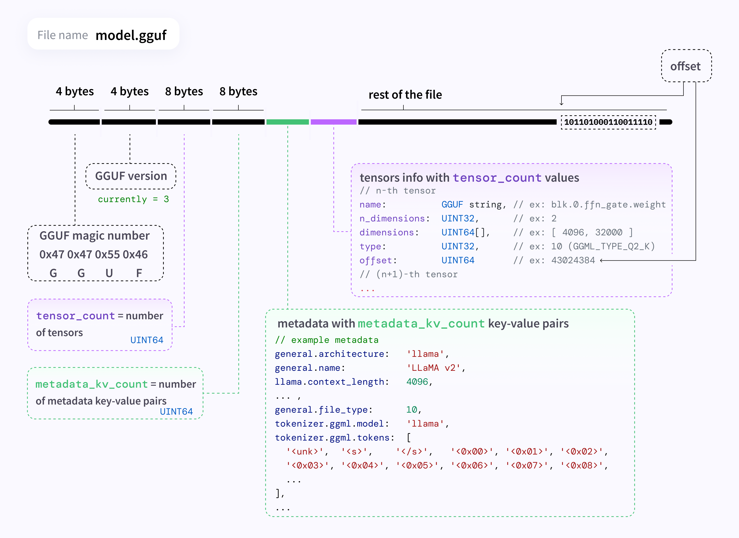
GGUF is designed for scenarios where you need to balance the computational load across both CPU and GPU resources. This approach is particularly beneficial when VRAM is limited. GGUF can offload specific layers to the CPU, making it versatile for setups with mixed hardware capabilities. It works well with the LLaMA models and supports advanced features like offloading layers, making it more efficient for users who don’t have enough GPU memory.

GGUF Quantization Types

GGUFQuantizationType	Description
F32	32-bit standard IEEE 754 single-precision floating-point number.
F16	16-bit standard IEEE 754 half-precision floating-point number.
Q8_0	8-bit round-to-nearest quantization (q). Each block has 32 weights. Weight formula: w = q * block_scale. Legacy quantization method (not used widely as of today).
Q8_1	8-bit round-to-nearest quantization (q). Each block has 32 weights. Weight formula: w = q * block_scale + block_minimum. Legacy quantization method (not used widely as of today).
Q8_K	8-bit quantization (q). Each block has 256 weights. Only used for quantizing intermediate results. All 2-6 bit dot products are implemented for this quantization type. Weight formula: w = q * block_scale.
Q6_K	6-bit quantization (q). Super-blocks with 16 blocks, each block has 16 weights. Weight formula: w = q * block_scale(8-bit), resulting in 6.5625 bits-per-weight.
Q5_0	5-bit round-to-nearest quantization (q). Each block has 32 weights. Weight formula: w = q * block_scale. Legacy quantization method (not used widely as of today).
Q5_1	5-bit round-to-nearest quantization (q). Each block has 32 weights. Weight formula: w = q * block_scale + block_minimum. Legacy quantization method (not used widely as of today).
Q5_K	5-bit quantization (q). Super-blocks with 8 blocks, each block has 32 weights. Weight formula: w = q * block_scale(6-bit) + block_min(6-bit), resulting in 5.5 bits-per-weight.
Q4_0	4-bit round-to-nearest quantization (q). Each block has 32 weights. Weight formula: w = q * block_scale. Legacy quantization method (not used widely as of today).
Q4_1	4-bit round-to-nearest quantization (q). Each block has 32 weights. Weight formula: w = q * block_scale + block_minimum. Legacy quantization method (not used widely as of today).
Q4_K	4-bit quantization (q). Super-blocks with 8 blocks, each block has 32 weights. Weight formula: w = q * block_scale(6-bit) + block_min(6-bit), resulting in 4.5 bits-per-weight.
Q3_K	3-bit quantization (q). Super-blocks with 16 blocks, each block has 16 weights. Weight formula: w = q * block_scale(6-bit), resulting. 3.4375 bits-per-weight.
Q2_K	2-bit quantization (q). Super-blocks with 16 blocks, each block has 16 weight. Weight formula: w = q * block_scale(4-bit) + block_min(4-bit), resulting in 2.5625 bits-per-weight.
IQ4_XS	4-bit quantization (q). Super-blocks with 256 weights. Weight w is obtained using super_block_scale & importance matrix, resulting in 4.25 bits-per-weight.
IQ3_S	3-bit quantization (q). Super-blocks with 256 weights. Weight w is obtained using super_block_scale & importance matrix, resulting in 3.44 bits-per-weight.
IQ3_XXS	3-bit quantization (q). Super-blocks with 256 weights. Weight w is obtained using super_block_scale & importance matrix, resulting in 3.06 bits-per-weight.
IQ2_S	2-bit quantization (q). Super-blocks with 256 weights. Weight w is obtained using super_block_scale & importance matrix, resulting in 2.5 bits-per-weight.
IQ2_XS	2-bit quantization (q). Super-blocks with 256 weights. Weight w is obtained using super_block_scale & importance matrix, resulting in 2.31 bits-per-weight.
IQ2_XXS	2-bit quantization (q). Super-blocks with 256 weights. Weight w is obtained using super_block_scale & importance matrix, resulting in 2.06 bits-per-weight.
IQ1_S	1-bit quantization (q). Super-blocks with 256 weights. Weight w is obtained using super_block_scale & importance matrix, resulting in 1.56 bits-per-weight.
IQ4_NL	4-bit quantization (q). Super-blocks with 256 weights. Weight w is obtained using super_block_scale & importance matrix.
I8	8-bit fixed-width integer number.
I16	16-bit fixed-width integer number.
I32	32-bit fixed-width integer number.
I64	64-bit fixed-width integer number.
F64	64-bit standard IEEE 754 double-precision floating-point number.
IQ1_M	1-bit quantization (q). Super-blocks with 256 weights. Weight w is obtained using super_block_scale & importance matrix, resulting in 1.75 bits-per-weight.
BF16	16-bit shortened version of the 32-bit IEEE 754 single-precision floating-point number.

Practical Example

1. Cloning and Building Llama.cpp

Here, we clone the Llama.cpp repository and set it up for CUDA acceleration. After pulling the latest updates, we compile the project with LLAMA_CUBLAS=1 for enhanced GPU support.

!git clone https://github.com/ggerganov/llama.cpp
!cd llama.cpp && git pull && make clean && LLAMA_CUBLAS=1 make
!pip install -r llama.cpp/requirements.txt
!(cd llama.cpp && make)

Finally, we install the Python dependencies and build the project to prepare for model quantization.

2. Downloading the Pretrained Model

In this block, we define the model ID and download it from Hugging Face using Git LFS. The model’s name is extracted from the ID for use in later steps.

model_id = "Qwen/Qwen2-1.5B-Instruct"
model_name = model_id.split('/')[-1]

# download model
git lfs install
git clone https://huggingface.co/{model_id}

This prepares the model files needed for conversion and quantization.

3. Converting the Model to FP16

Here, we convert the downloaded model to FP16 format using the Llama.cpp conversion script. This step is crucial as FP16 is the required format before further quantization into the GGUF format.

fp16 = f"{model_name}/{model_name.lower()}.fp16.bin"
!python llama.cpp/convert_hf_to_gguf.py {model_name} --outtype f16 --outfile {fp16}

4. Running the Quantization

In this block, we quantize the model using Llama.cpp’s quantization tool. We specify a quantization method like q4_k_m, which is optimized for a good balance between memory efficiency and accuracy. Other recommended methods include q5_k_m, q6_k, and q8_0 with the latter being an 8-bit quantization that is nearly lossless compared to the original model weights. The resulting GGUF file is ready for inference.

method = "q4_k_m"
qtype = f"{model_name}/{model_name.lower()}.{method.upper()}.gguf"
!./llama.cpp/llama-quantize {fp16} {qtype} {method}

5. Testing the Quantized Model

Finally, we run a test using the quantized model with a sample prompt. The model’s output is generated and evaluated using Llama.cpp’s CLI. This test demonstrates how well the quantized model retains performance despite reduced precision, allowing us to check its practical response quality.

!./llama.cpp/llama-cli -m {qtype} -n 128 --repeat_penalty 1.0 --color -i -r "User:" -f /content/llama.cpp/prompts/chat-with-bob.txt

4. EXL2 Quantization

EXL2 is an optimized quantization approach aimed at improving both inference speed and computational efficiency. While less common than methods like GPTQ, EXL2 focuses on reducing latency during inference by optimizing weight quantization and activation functions. It’s particularly useful for deployments where low-latency responses are critical, such as real-time applications.

Practical Example

1. Cloning and Installing ExLlamaV2

We start by cloning the ExLlamaV2 repository and installing its requirements. This package provides tools for model quantization and inference, specifically optimized for speed and memory efficiency.

!git clone https://github.com/turboderp/exllamav2
!(cd exllamav2 && pip install -r requirements.txt && pip install .)

2. Downloading the Pretrained Model

Next, we define the model ID and download it using Git LFS from Hugging Face. The model name is extracted for use in later steps.

model_id = "Qwen/Qwen2-1.5B-Instruct"
model_name = model_id.split('/')[-1]

# download model
git lfs install
git clone https://huggingface.co/{model_id}

3. Running the Quantizer with 4-bit Precision

In this step, we run the ExLlamaV2 quantization script with a bitrate of 4.0. The model files are specified as input, and the output is saved in a temporary directory. This process applies 4-bit quantization to the model weights, enabling efficient inference with reduced resource usage.

!mkdir temp
!python exllamav2/convert.py \
    -i {model_name} \
    -o temp/ \
    -cf {model_name}-exl2/{quant_bpw}bpw/ \
    -b {quant_bpw}

4. Testing the Quantized Model

Finally, we test the quantized model using the ExLlamaV2 inference script.

!python exllamav2/test_inference.py -m {model_name}-exl2/{quant_bpw}bpw -p "What is quantization ?"

A sample prompt ("What is quantization?") is passed to the model to evaluate its performance and verify the output quality after quantization.

5. AWQ Quantization

AWQ (Activation Weight Quantization) is another post-training quantization method similar to GPTQ but optimized for better performance on non-GPU setups, like laptops or Macs. It is particularly beneficial when using activation reordering, which can enhance accuracy even when the quantization data differs from the inference dataset. AWQ tends to be faster and more effective in such contexts compared to GPTQ, making it a popular choice for varied hardware environments.

Practical Example

1. Installing AutoAWQ Library

We start by installing the autoawq library, which is specifically designed for quantizing models using the AWQ method. This package is crucial for performing weight quantization and optimizing model inference.

pip install autoawq

2. Loading the Pretrained Model and Tokenizer

Next, we load the pretrained model using AutoAWQForCausalLM with options for reducing memory usage on the CPU.

from awq import AutoAWQForCausalLM
from transformers import AutoTokenizer

pretrained_model_dir = "Qwen/Qwen2-1.5B-Instruct"

model = AutoAWQForCausalLM.from_pretrained(
    pretrained_model_dir, **{"low_cpu_mem_usage": True, "use_cache": False}
)
tokenizer = AutoTokenizer.from_pretrained(pretrained_model_dir, trust_remote_code=True)

The tokenizer is also loaded, with trust_remote_code=True to allow loading custom configurations and scripts from the model’s repository.

3. Quantizing the Model Here, we define the quantization configuration with settings like:

• zero_point: Enables zero-point quantization.
• q_group_size: Set to 128 for better balance between speed and accuracy.
• w_bit: Configured to 4-bit quantization.
• version: Specifies the quantization strategy (like "GEMM").

# quantize the model
quant_config = { "zero_point": True, "q_group_size": 128, "w_bit": 4, "version": "GEMM" }
model.quantize(tokenizer, quant_config=quant_config)

These settings are used to quantize the model, adapting it for efficient inference while maintaining model quality.

4. Saving the Quantized Model

In this step, the quantized model and tokenizer are saved to a specified directory. This allows for easy reloading and deployment of the quantized model in future sessions.

quantized_model_dir = "Qwen2_AWQ"
model.save_quantized(quantized_model_dir)
tokenizer.save_pretrained(quantized_model_dir)

5. Loading and Testing the Quantized Model

Finally, we load the quantized model onto the first GPU (cuda:0) and set up a chat-like prompt using the tokenizer. The inputs are tokenized, moved to the GPU, and passed to the model for generating a response.

model = AutoAWQForCausalLM.from_quantized(quantized_model_dir, device="cuda:0") # loads quantized model to the first GPU
tokenizer = AutoTokenizer.from_pretrained(pretrained_model_dir)


prompt = tokenizer.apply_chat_template(
            [{"role": "system", "content": "You are a helpful assistent"} , 
            {"role": "user", "content": "What is Quantization ?"}  ],
            tokenize=False,
            add_generation_prompt=True,
)

inputs = tokenizer(prompt, return_tensors="pt")
inputs.to("cuda:0") # loads tensors to the first GPU

outputs = model.generate(**inputs, max_new_tokens=32)
response = tokenizer.decode(outputs[0], skip_special_tokens=True)

print(response)

The output is then decoded and printed, allowing us to observe how the quantized model performs in a practical scenario.

---

Understanding and applying various quantization techniques like Bits-and-Bytes, AWQ, GPTQ, EXL2, and GGUF is essential for optimizing model performance, particularly in resource-constrained environments. Each method offers unique advantages and challenges, making it crucial to select the right approach based on specific needs. By exploring these techniques hands-on, you can gain deeper insights into how quantization impacts model efficiency, accuracy, and deployment.

For a more visual understanding of the quantization topic, I recommend checking out this blog: Maarten Grootendorst's Quantization Guide.

---